Research Article
Estimating Physiological Dose Optima in Plant Radiohormesis Through Censoring-Aware Hierarchical Bayesian Modeling
- 1 Institute of Energy and Nuclear Research (IPEN), University of São Paulo (USP), São Paulo, São Paulo, Brazil
- 2 School of Education, Humanities and Languages (ESEHL), International University Center (UNINTER), Curitiba, Paraná, Brazil
- 3 Center for Nuclear Energy in Agriculture (CENA), University of São Paulo (USP), Piracicaba, São Paulo, Brazil
Corresponding author: Luis Felipe Medeiro Alves, Institute of Energy and Nuclear Research (IPEN), University of São Paulo (USP), São Paulo, Brazil. Email: alves.luis@alumni.usp.br
Abstract
Background: Low doses of ionizing radiation can enhance germination and early seedling vigor in many plant species, but dose–response curves are often measured over a narrow dose range. As a result, the empirical dose of maximal stimulation () is frequently recorded at the limits of that range, so estimates that treat those boundary values as exact can be biased.
Objectives: Using dose–response data from Nicotiana tabacum, a censoring-aware framework is developed to obtain biologically interpretable estimates of across developmental traits.
Methods: The approach combines a censored regression formulation with a hierarchical Bayesian model that partially pools information across varieties and developmental traits while preserving the differences between them.
Results: Posterior inference showed a consistent pattern: germination and early seedling traits had lower optimal doses, whereas biomass-related traits were shifted into the upper part of the tested range, which suggests distinct radiosensitivity regimes across developmental stages.
Conclusion: The sample is small, so the framework is presented as a means of estimating stimulation optima together with the uncertainty that boundary effects induce, to guide the design of pre-sowing irradiation trials.
Keywords: censored regression, dose–response, hierarchical Bayesian model, Nicotiana tabacum, optimal dose, radiohormesis, seed priming
1. Introduction
Low-dose radiation responses consistent with hormesis have been reported in several plant systems, including seed-priming studies 1–3. Exposure of seeds to low doses of ionizing radiation may enhance early vigor, accelerate germination, strengthen antioxidant capacity and modulate subsequent stress responses 4–11. The expected biological pattern is biphasic: stimulation at low doses followed by loss of benefit or inhibition as dose increases. This pattern can be represented by several empirical and semi-mechanistic dose–response functions, including quadratic models and the Brain–Cousens hormetic function 12–17. Across these formulations, the operationally important quantity is the dose at which the measured physiological response reaches its maximum. Reliable estimation of therefore underpins the design of reproducible seed-priming protocols, a problem that has been approached empirically across a wide range of crop and model species 18–30.
1.1 Current Predictive Frameworks and Their Limitations
A meta-regression model was recently introduced to predict the empirical optimum (the observed ) from high-level covariates such as variety, physiological endpoint, and measurement time 31. Although this model showed that radiosensitivity patterns are structured and predictable, the approach fits those optima by ordinary least squares (OLS). OLS assumes that the response entering the regression is the quantity of interest, observed exactly, with errors that are independent and homoscedastic and, for the usual interval estimates, normal. Censoring is a property of how the optimum is observed. When a fitted optimum is reported at the edge of the tested range, the recorded number is a bound on the quantity of interest rather than the quantity itself, and the exact-observation assumption is the one that fails.
In practice, seed-priming experiments are commonly constrained to a narrow dose range; the experiment re-analyzed here used 0–20 Gy 32. When the true optimum lies below or above the tested range, curve-fitting procedures return a boundary value (0 Gy or 20 Gy), yielding a censored estimate of . The OLS model treats these censored values as precise observations, leading to regression coefficients that are biased downward or upward depending on the censoring direction and frequency. These biases propagate into dose recommendations.
1.2 Censoring as a Structural Feature of Irradiation Experiments
Boundary optima are an intrinsic consequence of experimental design. For physiologically vigorous genotypes, the true optimum may exceed 20 Gy, while sensitive genotypes may peak at doses below the minimum tested. Writing for the dose at which the underlying response surface peaks, for the tested range, and for the optimum a curve fit reports, these outcomes are
An optimum recorded at is right-censored and one recorded at is left-censored; Section 3 gives the full observation model and the likelihood it implies. The distribution of censoring is itself informative: varieties whose optima reach the upper boundary more often may have higher intrinsic oxidative resilience or slower lesion accumulation. Censoring therefore has to be incorporated into inference.
1.3 A Statistical Framework for Latent Dose Estimation
To address these limitations, this work introduces: (i) a Tobit model that accounts for censoring in a frequentist framework, adjusting estimates of latent optima and regression parameters for boundary effects; and (ii) a hierarchical Bayesian model (HBM) that incorporates censoring directly into the likelihood, partially pools information across varieties and endpoints, and delivers posterior distributions of latent radiosensitivity. The Bayesian formulation represents variability across varieties and endpoints explicitly, quantifies posterior uncertainty, and remains consistent with redox kinetic theory.
1.4 Biological and Agronomic Relevance
Improved estimation of has direct practical relevance because seed-priming protocols must balance stimulation against the risk of entering the inhibitory region of the dose–response curve. A statistical model that accounts for boundary optima can help distinguish between an experimentally observed maximum and a maximum that may have been truncated by the dose window. This distinction is especially important when different physiological endpoints respond over different time scales. Endpoint identity already accounts for part of the variation in the empirical optima of this experiment 31, and the analysis below places the early germination and seedling traits lower in the tested range than the biomass traits. A censoring-aware model can therefore support more cautious, endpoint-specific experimental designs.
The remainder of the manuscript sets out the steps from the censored observations to latent-dose inference and endpoint-specific dose summaries.
2. Materials and Existing Models
2.1 Dataset Structure and Preprocessing
The dataset comprises fitted optima () from multiple dose–response curves across tobacco cultivars: Burley (BY), Dark (DK), and Virginia (VA). The underlying irradiation experiment and its dose–response measurements are reported in full by Alves et al. 32; the present work re-analyzes those measurements and introduces no new observations. The same measurements were previously fitted per variety and endpoint with quadratic and Brain–Cousens models, and the resulting optima summarized by the meta-regression described below 31; the optima used here are recomputed by quadratic fits alone, as set out in Section 3.
The physiological endpoints are the developmental traits recorded in that experiment, summarized into the nine endpoints analyzed here. Three of the traits are time-course measurements: germination, hypocotyl emergence, and cotyledon expansion, each recorded on days 3, 5, 7, and 9 after sowing as a count out of the 50 seeds sown per replicate. Each is summarized in two ways, giving six endpoints: the day-9 count, which is the terminal value of that trait, and the sum of the four counts recorded for it. The remaining three are plantlet biomass at two weeks, plantlet biomass at four weeks, and the increment between them. Table 1 lists all nine.
All optima were extracted by least-squares quadratic fits to the dose-wise means over a common dose range of 0–20 Gy, by the procedure set out in Section 3.
After constructing dose–response summaries as described below, the meta-dataset used for regression comprises optimal-dose estimates , each corresponding to a specific combination of variety, endpoint, and time scale within the dose window Gy. As detailed in Section 3, two of these optima are formally right-censored at 20 Gy, while the remainder lie strictly inside the experimental range.
2.2 Baseline OLS Model
The existing predictive model 31 is:
where and the predictors code varieties, physiological endpoints, and measurement time.
OLS assumes complete observations and ignores censoring, which structurally biases the estimates when boundary optima are present.
2.3 Mechanistic Context: Redox–Lesion Kinetics
Generalized kinetic models describing reactive oxygen species (ROS) production (), antioxidant pools (), and lesion load () yield a scaling relation of the form
in the regime , where is the fidelity-collapse threshold and summarize adaptive and damaging processes. The exponent is negative because raising adaptive capacity relative to damage moves the optimum to a higher dose, so the ratio decreases. The lesion load is the effective burden of persistent oxidative lesions, that is, the macromolecular damage left after repair; that model keeps it deliberately unresolved, aggregating the damage classes rather than tracking DNA strand breaks, oxidized bases, and lipid peroxidation products separately 12. A predictive model for should remain compatible with this mechanistic structure so that its parameters can, at least qualitatively, be related to redox–lesion kinetics 12, 31, 33.
| Endpoint | Description | Time scale | opt | Censored (20 Gy) |
|---|---|---|---|---|
| Germ_D9 | Germinated seeds at day 9 | 9 days | 3 | 0 |
| Germ_AUC | Sum of germinated-seed counts | 3–9 days | 3 | 0 |
| Hypo_D9 | Hypocotyl emergence at day 9 | 9 days | 3 | 0 |
| Hypo_AUC | Sum of hypocotyl-emergence counts | 3–9 days | 3 | 0 |
| Coty_D9 | Cotyledon expansion at day 9 | 9 days | 3 | 0 |
| Coty_AUC | Sum of cotyledon-expansion counts | 3–9 days | 3 | 0 |
| Plantlet biomass at 2 weeks | 2 weeks | 3 | 1 | |
| Plantlet biomass at 4 weeks | 4 weeks | 3 | 0 | |
| Biomass increment () | 4 weeks | 3 | 1 |
3. Methodology
This section sets out the statistical pipeline used to obtain estimates of the physiological optimum dose under censoring. The analysis proceeds in three stages. First, endpoint-specific dose–response summaries are constructed from the raw experimental data and a preliminary estimate of is extracted for each variety-by-endpoint combination by quadratic regression. Second, censoring is formalized through a classical Tobit-type latent variable formulation, which clarifies why ordinary least squares applied to the observed optima is biased in the presence of boundary effects. Third, a hierarchical Bayesian model with a logit–normal latent structure and censoring-aware likelihood is specified, yielding posterior distributions for latent optima and for variety- and endpoint-specific effects. Logit–normal here means that a linear predictor on the real line is given a normal distribution and mapped into the tested dose interval by the inverse logit, so the induced distribution of the latent optimum is supported on and on no value outside it. The mapping is stated below, under Logit–Normal Mapping to the Dose Interval.
As above, the lower and upper experimental bounds of the irradiation range are denoted by and . In the present experiment Gy and Gy 32.
3.1 Construction of Endpoint-Specific Optima
3.1.1 Time-Course Endpoints
For germination, hypocotyl, and cotyledon traits, measurements were taken at four time points: day 3, day 5, day 7, and day 9 after sowing. Let
denote the count recorded for treatment at time point days, out of the 50 seeds sown per replicate. Two families of dose–response endpoints are derived for each trait:
- 1. Terminal value at day 9:
the value of that physiological variable at the end of the time course.
- 2. Cumulative sum over the time course (labeled AUC):
Summing the four recorded counts avoids interpolating between observation days. The label AUC is retained for continuity with the endpoint names used in the source experiment 32, although the quantity is a sum of counts rather than an integral.
For each trait and treatment two derived endpoints are obtained, labeled generically as
3.1.2 Biomass Endpoints
The biomass table records plantlet weight at two weeks (), plantlet weight at four weeks (), and the increment . These are treated as additional scalar endpoints:
3.1.3 Long-Format Endpoint Table
All derived endpoints are assembled into a single long-format table. Each row corresponds to a specific combination of variety, dose, replicate (where applicable), physiological endpoint, and associated time scale (9 days for the terminal endpoints, 3-9 days for the cumulative-sum endpoints, 2 weeks for , and 4 weeks for and ). Formally, each row is
where is the variety, is the physical dose, is the replicate label (or missing for pooled biomass), is the endpoint name, is the associated temporal scale, and is the measured value.
3.1.4 Dose–Response Means per Variety, Endpoint, and Dose
Because multiple replicates are available at each dose for most endpoints, dose-wise means are computed to obtain one dose–response curve for each combination of variety and endpoint. For fixed , let be the set of rows corresponding to that triplet, and define
The resulting table has one record for each .
3.2 Quadratic Approximation and Preliminary
For each combination the quadratic model
is fitted by ordinary least squares over the available doses . The fitted quadratic has vertex
The sign of is tested first. If the quadratic has no interior maximum and the optimum falls on a boundary; the two boundary predictions are compared, is set to the boundary with the higher predicted response, and the observation is marked as censored.
If the quadratic is concave and is its maximum. When the vertex is taken as the preliminary optimum and labeled uncensored. When it falls outside the interval the optimum is placed at the nearer boundary and marked as censored:
This yields a meta-dataset in which each row corresponds to a variety , endpoint , and time scale, with an associated preliminary optimum and an indicator flag specifying whether the optimum is censored at or . This table serves as input for the subsequent censored regression analysis.
3.3 Censored Regression (Tobit Model)
3.3.1 Latent Variable Formulation
Let denote the preliminary optimum for observation . When the true optimum lies outside the experimental range, is censored at or . An unobserved latent variable is introduced, with
where is a vector of predictors comprising dummy variables for variety and endpoint together with the time of measurement, is a vector of regression coefficients, and is the residual variance.
3.4 Observation Mechanism and Censored Likelihood
The observed optimum is related to the latent value via
With and denoting the normal density and cumulative distribution function with mean and variance , the likelihood contributions are
for uncensored, left-censored, and right-censored sets . The full likelihood is
3.5 OLS as a Naïve Benchmark
A naïve OLS regression that treats as fully observed ignores censoring. Boundary optima are interpreted as exact, which induces bias: right-censored optima at are treated as if the true optimum were exactly , rather than somewhere beyond that point. The Tobit model explicitly accounts for this by treating boundary values as inequalities in the likelihood.
3.6 Hierarchical Bayesian Model (HBM)
The classical Tobit model does not explicitly represent hierarchical structure across varieties and endpoints, and it is not naturally framed for prediction with partial pooling. A hierarchical Bayesian model that generalizes the Tobit formulation is therefore adopted.
3.7 Hierarchical Structure and Linear Predictor
Let denote the variety associated with observation and denote the physiological endpoint. Random effects for varieties and endpoints and a time effect are introduced:
where is a variety-specific intercept, is an endpoint-specific intercept, is the time covariate after centering and scaling, and is a fixed slope.
Because each endpoint is observed on a single time scale, the time covariate is a deterministic function of endpoint identity. The coefficient is therefore not identified as a dose–time relationship and is not interpreted as one; it acts as a grouping of endpoints by measurement scale, which the hierarchical prior shrinks less strongly than the individual endpoint effects.
3.8 Logit–Normal Mapping to the Dose Interval
The physiological optimum dose is constrained to lie in . is therefore mapped to the dose scale by
with
This yields a logit–normal prior structure for the latent optimum, so that by construction.
3.9 Observation Model with Additive Noise
Conditional on , the preliminary optimum is modeled as
subject to the same censoring mechanism at and :
where and are the standard normal density and distribution functions.
3.10 Hierarchical Priors
Hierarchical priors are assigned to the random effects:
with hyperpriors
The time effect is assigned a weakly informative prior
after centering and scaling the time covariate. The residual standard deviation is modeled as
3.11 Full Joint Distribution
Collecting the model parameters in and denoting , the joint posterior is
with .
3.12 Posterior Inference via Hamiltonian Monte Carlo
Posterior inference is performed using the No-U-Turn Sampler (NUTS) implemented in PyMC. Four independent Markov chains were run, each with 1500 tuning iterations at a target acceptance probability of 0.95 followed by 2000 post-tuning draws, yielding 8000 posterior samples. Sampling was well behaved: no divergent transitions were recorded, the split- statistic equaled 1.00 for every parameter, and the smallest bulk effective sample size was 2901 of the 8000 draws. The sampler produced an Inference Data object containing posterior draws, sampling statistics, and the observed data.
Posterior summaries for variety and endpoint effects are obtained by transforming draws of through the logistic function to obtain draws of for each observation and aggregating across the relevant groups.
3.13 Model Comparison and Information Criteria
Three models are compared:
- 1. a naïve OLS regression that ignores censoring;
- 2. a classical Tobit regression with right-censoring at Gy; and
- 3. the hierarchical Bayesian model described above.
Maximized log-likelihoods were computed for the OLS and Tobit models. The OLS regression yielded a maximized log-likelihood of , whereas the right-censored Tobit model yielded a maximized log-likelihood of , so
The two fits carry the same regression parameters and the same residual scale and differ only in how the two boundary observations enter the likelihood; they are therefore not nested, and no likelihood-ratio test applies. The comparison establishes only that the difference is of the order of one hundredth of a log-likelihood unit: with this sample size and this censoring pattern, treating the two boundary values as inequalities rather than as exact observations leaves the maximized likelihood essentially unchanged. The case for the censored formulation therefore rests on its structure rather than on a measured gain in fit.
For the hierarchical Bayesian model the Watanabe–Akaike Information Criterion (WAIC) and approximate leave-one-out cross-validation using Pareto-smoothed importance sampling (PSIS–LOO) were computed from the pointwise censored-normal log-likelihood. Writing for the log-likelihood at observation and posterior draw , the log pointwise predictive density is
from which WAIC estimates the expected log predictive density by subtracting an effective number of parameters , obtained from the posterior variance of the pointwise log-likelihoods:
On the log (elpd) scale reported by ArviZ, the hierarchical model gave
so and on the deviance scale. ArviZ issued a diagnostic warning that for four observations the posterior variance of the log predictive density exceeded 0.4, the largest being 1.16, so WAIC should be read with caution for those points. They are the two censored biomass optima, the two-week biomass optimum of DK, and the low hypocotyl-AUC optimum of VA.
PSIS–LOO approximates exact leave-one-out cross-validation using importance weights stabilized by a generalized Pareto distribution. For the hierarchical model, on the same elpd scale,
consistent with the WAIC estimate ( versus , well within either standard error). The Pareto shape parameter exceeded 0.70 for one of the 27 observations, the two-week biomass optimum of VA at , with no value above 1. The importance-sampling approximation is therefore reliable apart from that single point, whose leave-one-out contribution should be treated as approximate.
The effective number of parameters is small relative to the sample size ( and against ), which is what partial pooling of three variety effects and nine endpoint effects should produce, and the two criteria agree to within their standard errors. They indicate that the model is not overfitting the 27 optima, subject to the single influential observation noted above. Both flags fall on the censored and the most extreme optima, which is where the sample is thinnest. WAIC and PSIS–LOO were not computed for the OLS or Tobit models, and no numerical ranking of the three models is made. Table 2 collects the values.
| Model | |||||
|---|---|---|---|---|---|
| OLS (uncensored) | – | – | – | – | |
| Tobit (right-censored) | – | – | – | – | |
| HBM (censored, hierarchical) | – | 5.77 | 6.21 |
3.14 Reproducibility and Software
All analyses were performed in Python using the PyMC ecosystem for Bayesian modeling and ArviZ for posterior diagnostics and information criteria. The code used to construct the endpoint tables, fit the censored hierarchical models, and generate the figures is available from the corresponding author upon reasonable request and can be readily adapted to other dose–response datasets. The posterior reported here was drawn with a fixed random seed, so the figures and every quoted value regenerate exactly.
4. Results
This section presents the consequences of explicitly modeling censoring in the estimation of optimal stimulation dose () and reports the main features of the posterior structure obtained from the hierarchical Bayesian model (HBM). The information criteria for this dataset are well behaved: the effective numbers of parameters are small relative to the sample size ( and for ), and WAIC and PSIS–LOO agree to within their standard errors, with one influential observation carrying a Pareto- above 0.70. They are reported as evidence against overfitting rather than as a ranking of the three models.
4.1 Effects of Censoring on Regression Structure
A central objective of this study is to understand how censoring affects the regression structure linking varieties, physiological endpoints, and time to the dose of maximal stimulation. In the meta-dataset, 27 optima are available and two are formally right-censored at 20 Gy. Several additional optima lie close to the upper boundary and behave, in practice, like censored points.
In a naïve OLS analysis, all boundary values are treated as exact optima. This forces the regression surface to accommodate artificial constraints and tends to compress apparent differences between groups, particularly for endpoints whose fitted optima are at or near 20 Gy. The Tobit likelihood treats a boundary observation as an inequality on the dose scale,
In the hierarchical logit–normal model, by contrast, is constrained to the experimental interval , and right-boundary observations contribute through the upper-tail probability of the censored observation model. Thus, in both cases, a boundary value is not treated as an exact interior optimum.
In the hierarchical model, variety and endpoint effects are shrunk toward a global mean, but in a way that respects censoring: groups associated with boundary optima are not forced to share the same latent optimum as groups whose optima lie well inside the experimental range. This improves interpretability of differences across endpoints relative to the OLS benchmark.
4.2 Latent vs. Observed Optima
Observed optima arise from quadratic fits to noisy dose–response curves over a finite set of doses. Curves whose maxima are not well resolved within the tested range may therefore produce apparent optima near the upper boundary. By contrast, the hierarchical Bayesian model returns a posterior distribution for the underlying optimum within the experimental interval, integrating information across varieties and endpoints.
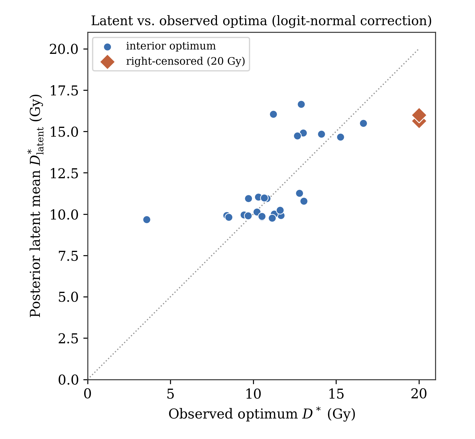
Figure 1 shows the effect. The latent estimates separate by endpoint class in a way the observed optima do not: the 18 early-vigor observations occupy 9.7 to 11.3 Gy and the nine biomass observations 14.7 to 16.7 Gy, a gap of 3.4 Gy with no overlap, whereas the observed optima of the two groups overlap heavily (3.6–13.0 Gy against 11.2–20.0 Gy). Within each band the latent value varies little with the observed one, so a least-squares line through the 27 pairs has slope 0.55 rather than 1: partial pooling replaces each individual optimum with the value implied by its variety and endpoint. The extreme values move most. The 3.6 Gy hypocotyl-AUC optimum of VA is placed at 9.7 Gy, and the two optima censored at 20 Gy at 15.6 and 16.0 Gy. The censored pair falls in the upper quarter of the tested window, which is the closest the logit–normal mapping can place an optimum that the data bound only from below.
4.3 Posterior Predictive Checks
Posterior predictive checks (PPCs) assess absolute model adequacy. For each posterior draw a replicated dataset was generated by sampling latent optima from the logit–normal structure and applying the censored observation model. Four statistics of each replicate were then compared with the observed data: the mean of the 27 optima, their standard deviation, the number right-censored at 20 Gy, and the height of the tallest 2 Gy histogram bin. The first two test location and spread, the third tests whether the model reproduces boundary censoring at the observed rate, and the fourth tests how tightly the interior optima are concentrated.
The model reproduces both the location and the overall spread of the optima. The observed had mean 11.84 Gy and standard deviation 3.38 Gy; across 1000 replicated datasets the mean of the replicate means was 11.95 Gy, with standard deviation 0.75 Gy across replicates, against the Gy that the observed sample implies for a mean of 27 optima. The within-replicate standard deviation averaged 3.85 Gy, with 95% interval 2.67 to 5.17 Gy, so the observed 3.38 Gy falls inside the predictive range.
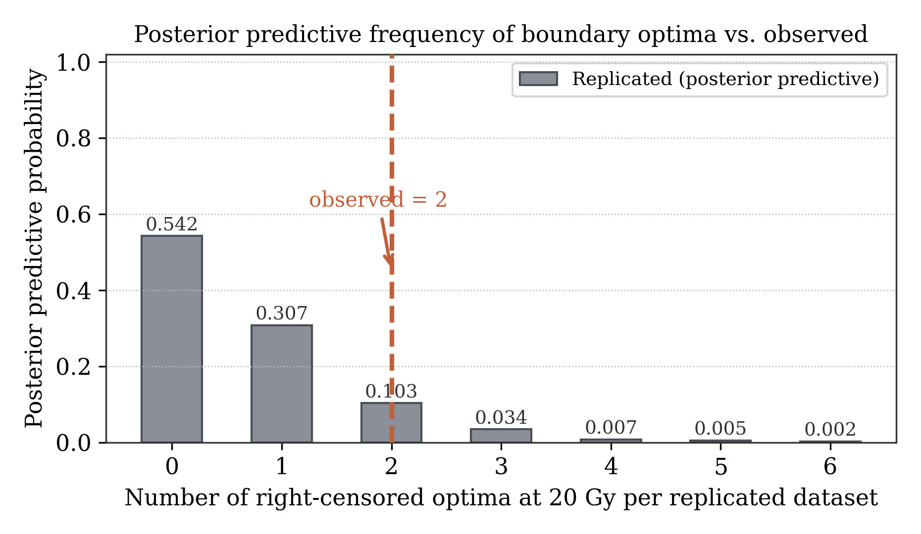
The frequency of boundary optima is reproduced as well. Two optima were right-censored at 20 Gy in the data; across replicates the censored count had mean 0.68 (standard deviation 0.93; central 95% interval ), two or more arose in 15.1% of replicated datasets and none in 54.2% (Figure 3), so the observed count of two lies inside the predictive distribution. This follows from treating those two observations as lower bounds rather than as exact values. The censored likelihood places their latent optima at 15.6 and 16.0 Gy. At the posterior mean of the observation noise, Gy, a latent optimum that close to the boundary carries a replicated draw past 20 Gy with appreciable probability.
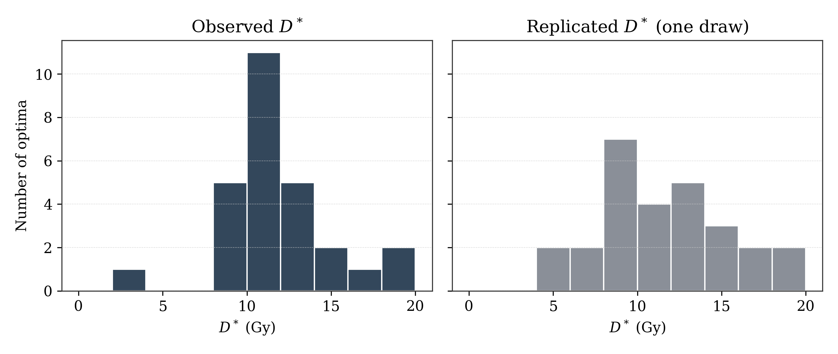
The model does not reproduce the concentration of the interior optima. Eleven of the 27 observed optima fall in the single 2 Gy interval from 10 to 12 Gy (Figure 2), whereas the tallest bin of a replicated dataset holds 7.1 optima on average, with 95% interval 5 to 10, and reaches eleven in 1.9% of replicates. The observation noise required to accommodate the extremes of this sample is therefore larger than the dispersion of its center, and the interior optima are spread more evenly than in the data. The interval estimates in Tables 3 and 4 are consequently more likely to be too wide than too narrow.
One limitation is structural, the logit–normal mapping constrains every latent optimum to lie strictly inside Gy, so an endpoint whose true optimum lies beyond the tested range can be placed near the upper boundary but never past it. For the biomass endpoints, with posterior means from 15.0 to 16.2 Gy, the model should therefore not be read as evidence that the optimum lies within 20 Gy; the cautious reading is that the tested window may be incomplete and that a wider dose range is needed to resolve the upper tail.
4.4 Empirical Structure of BY Optima
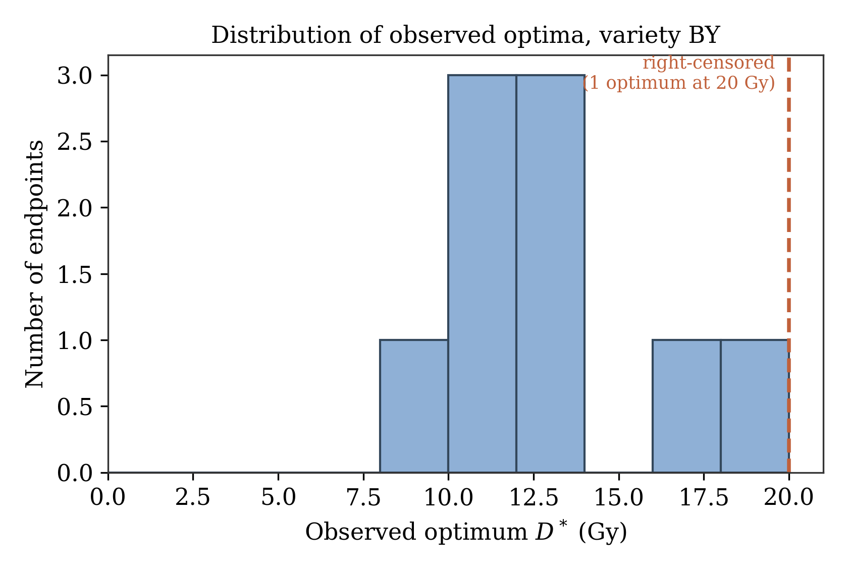
Before the hierarchical summaries, the empirical optima for variety BY are examined on their own. Figure 4 displays the distribution of observed values obtained from quadratic fits, showing a concentration around mid-range doses and no left-censored values, with one right-censored observation at 20 Gy.
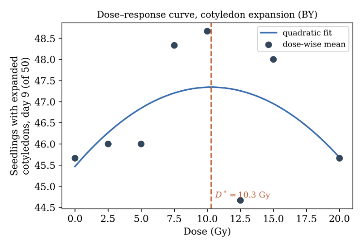
Figure 5 gives one dose–response curve in full, cotyledon expansion at day 9 in BY, and shows the basis of a single extracted optimum. The dose-wise means occupy a range of four seedlings out of 50, they fall and rise again above the fitted maximum, and the quadratic accounts for a quarter of their variation (), so the vertex at 10.3 Gy is a weakly determined summary of that curve. This is the uncertainty the hierarchical model carries, and the reason the individual optima are pooled rather than interpreted separately.
4.5 Qualitative Patterns Across Endpoints and Varieties
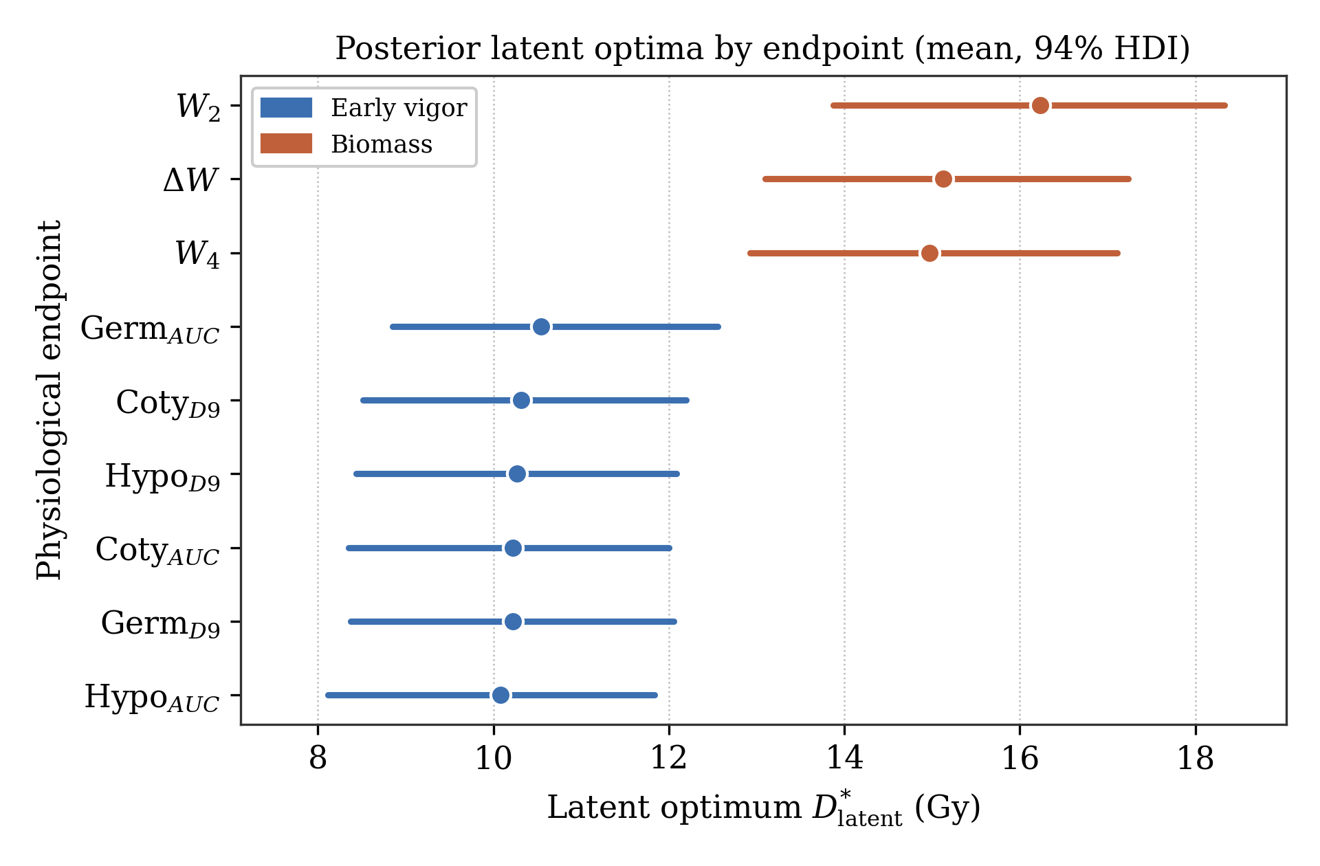
Figure 6 presents posterior estimates of the latent optimal dose for each physiological endpoint, with posterior means and 94% highest-density intervals, and Table 3 gives the same summaries numerically. Early-stage traits (germination, hypocotyl, cotyledons) have posterior means from 10.08 to 10.55 Gy, close to the midpoint of the 0–20 Gy window, whereas biomass-related endpoints (, , ) sit higher, from 14.97 to 16.23 Gy, and include right-censored contributions. Averaged across varieties, the biomass optima exceed the early-vigor optima by 5.17 Gy, with 94% highest-density interval 2.89 to 7.47 Gy, and the posterior probability that the biomass group carries the higher optimum is 0.9998.
| Endpoint | Mean (Gy) | 94% HDI lower (Gy) | 94% HDI upper (Gy) |
|---|---|---|---|
| Coty_AUC | 10.23 | 8.35 | 12.00 |
| Coty_D9 | 10.31 | 8.52 | 12.20 |
| 15.13 | 13.10 | 17.24 | |
| Germ_AUC | 10.55 | 8.85 | 12.56 |
| Germ_D9 | 10.22 | 8.38 | 12.06 |
| Hypo_AUC | 10.08 | 8.12 | 11.84 |
| Hypo_D9 | 10.27 | 8.44 | 12.09 |
| 16.23 | 13.87 | 18.33 | |
| 14.97 | 12.92 | 17.11 |
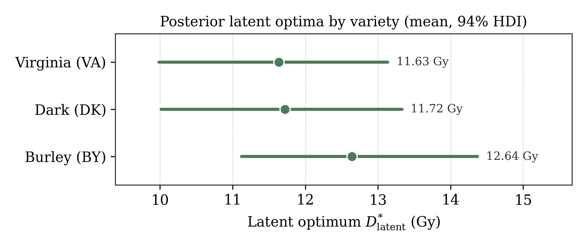
| Variety | Mean (Gy) | 94% HDI lower (Gy) | 94% HDI upper (Gy) |
|---|---|---|---|
| BY | 12.64 | 11.12 | 14.37 |
| DK | 11.72 | 10.01 | 13.33 |
| VA | 11.63 | 9.98 | 13.14 |
At the variety level, Figure 7 and Table 4 show that the three Nicotiana cultivars have overlapping posterior intervals, with latent optima between 11.63 and 12.64 Gy. Genotypic differences in the location of the hormetic peak are therefore modest compared with endpoint-driven variation.
| Endpoint class | Posterior pattern | Suggested implication for future experiments |
|---|---|---|
| Germination, hypocotyl, and cotyledon endpoints | Posterior means occur near 10–11 Gy, with 94% intervals spanning roughly 8 to 12.5 Gy. | Future studies focused on early vigor should use denser dose spacing between about 8 and 13 Gy, rather than concentrating only on the upper end of the range. |
| Biomass-related endpoints (, , and ) | Posterior means are higher, approximately 15–16 Gy, with intervals reaching 18.3 Gy at the upper end. | Future studies focused on biomass should sample densely from about 12 to 20 Gy and extend the upper dose range to 25–30 Gy, since the model can place an optimum near the tested boundary but not beyond it. |
| Variety-level effects | BY, DK, and VA show overlapping posterior intervals, with smaller differences than those observed among endpoint classes. | Dose optimization should prioritize the target physiological endpoint before making fine variety-level adjustments. |
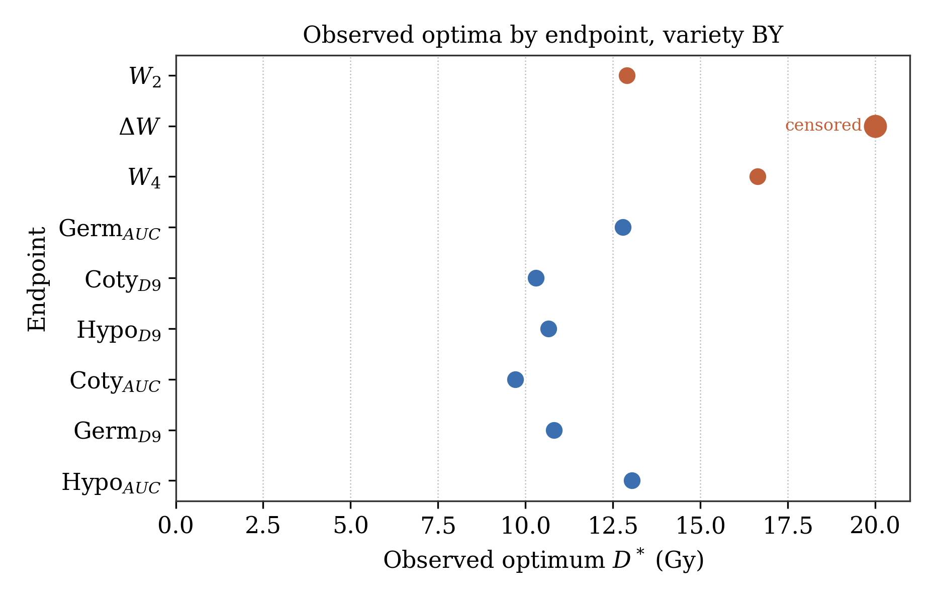
Finally, Figure 8 displays the observed optima for each endpoint in BY. Vigor-related endpoints tend to have interior maxima at lower doses, whereas the biomass endpoints shift upward and include the right-censored optimum at 20 Gy. The two sets interleave in this variety: the hypocotyl-AUC optimum at 13.0 Gy lies above the two-week biomass optimum at 12.9 Gy. The raw pattern therefore agrees with the hierarchical inference in direction. Table 5 sets out what these posterior patterns imply for the design of subsequent experiments.
4.6 Summary of Main Patterns
The censored hierarchical Bayesian model characterizes the optimal dose estimates of multiple traits under boundary censoring. It corrects the main conceptual deficiency of OLS (treating boundary optima as exact), reveals endpoint-specific differences that agree with the raw data, and yields posterior distributions that can be used in downstream decision-support tools. At the same time, the small sample size and the limited number of censored points indicate that model-based conclusions should be interpreted cautiously, especially for extrapolation beyond the observed dose range. The results should therefore be viewed as a proof-of-concept application of censored hierarchical modeling to plant radiohormesis.
5. Discussion
The main aim of this work was to examine how censoring at the experimental dose boundaries affects inference on the dose of maximal stimulation and to propose a correction suitable for small, structured plant radiobiology datasets. Within the context of this experiment, the censored hierarchical framework developed here makes three contributions: (i) it treats boundary optima as censored rather than exact values; (ii) it partially pools information across varieties and endpoints; and (iii) it returns posterior distributions that can be interpreted in relation to endpoint-specific radiosensitivity.
Introducing a latent optimum addresses a key limitation of a naïve OLS analysis. In OLS, an estimated optimum at 20 Gy is treated as if the physiological maximum were exactly 20 Gy. In the censored formulation, the same observation contributes information that the latent optimum is supported near the upper boundary of the tested range. This distinction is important because the experimental design may truncate the observable peak of the response curve.
The hierarchical Bayesian formulation partially pools information across varieties and endpoints, which is useful here because each variety–endpoint combination contributes only one estimated optimum. The model thus avoids treating each subgroup as completely independent while still allowing endpoint-level differences to emerge when supported by the data.
The logistic mapping from the latent linear predictor to the experimental dose interval (0,20) Gy enforces a mechanistically sensible constraint. The physiologically relevant optimum must lie within the explored dose range, and the logit–normal structure ensures this by construction. At the same time, a shift on the latent scale has a monotone effect on the position of the optimum within the window, making it straightforward to interpret the direction and relative magnitude of variety and endpoint effects.
When summarized by the dose of maximal stimulation, the three Nicotiana tabacum varieties show broadly similar radiosensitivity. The posterior intervals for Burley (BY), Dark (DK), and Virginia (VA) overlap, and the variety-level optima cluster between 11.6 and 12.6 Gy (Table 4), so under these conditions endpoint identity separates the optima more than genotype does.
The endpoint-level pattern carries the biological signal. Germination, hypocotyl emergence, and cotyledon expansion peak at lower doses (posterior means from 10.1 to 10.6 Gy), whereas the three biomass endpoints have higher optima (from 15.0 to 16.2 Gy). A redox interpretation accounts for this ordering. Low-dose irradiation raises the intracellular flux of reactive oxygen species (ROS), which at moderate concentrations act as signaling intermediates. They oxidize redox-sensitive transcription factors, feed into mitogen-activated protein kinase cascades and hormonal cross-talk, and induce the antioxidant machinery (superoxide dismutase, catalase, and ascorbate peroxidase) that sets the operating redox point of the cell 4, 5, 15. Stimulation gives way to inhibition once ROS production outpaces this induced scavenging capacity and oxidative lesions accumulate faster than they are repaired. The redox–lesion scaling describes that balance 12, 31.
The endpoint contrast then follows from the time scale over which each trait integrates this balance. Germination and early seedling traits are measured within nine days, during a phase dominated by reserve mobilization, membrane repair, cell expansion, and the first divisions of the radicle and shoot meristems. These processes run while the ROS flux raised by irradiation is still high and the induced antioxidant response is still incomplete 15, so their benefit is exhausted at a comparatively low dose. Biomass at two and four weeks accumulates after the antioxidant system has had time to respond; delayed enzymatic adjustment, compensatory growth, and cumulative carbon allocation extend the net-beneficial regime to higher doses before damage dominates. On this reading the higher optima for , , and mark a distinct, later-integrating response regime, and they imply that early vigor and biomass accumulation are best served by different doses.
From an agronomic viewpoint, the results do not support a single universal irradiation dose for all seed-priming objectives. The posterior summaries place the early vigor traits near the middle of the tested interval and the biomass-related traits in its upper quarter. For early germination and seedling development, future experiments should include denser sampling between about 8 and 13 Gy. For biomass-related endpoints, the present data support dense sampling from about 12 to 20 Gy, and they argue for extending the upper range, for example to 25–30 Gy, so that the decline after the stimulatory region can be directly observed.
These ranges are recommendations for experimental design, derived from the posterior structure of the present dataset. Practical agronomic recommendations would require additional replication, more genotypes, validation under greenhouse or field conditions, and direct assessment of yield-related outcomes. The model nevertheless translates censored dose–response information into testable dose windows for subsequent seed-priming studies.
The posterior distributions also allow recommendations to be expressed as uncertainty intervals rather than as single point estimates. This is important for irradiation protocols because the practical cost of an excessive dose may be larger than the cost of applying a slightly suboptimal stimulatory dose. In future decision-support applications, posterior dose distributions could be combined with endpoint priorities, genotype information, and acceptable risk thresholds to select conservative dose ranges for experimental validation.
5.1 Limitations
The present analysis should be interpreted in light of several limitations. First, the meta-dataset contains only 27 variety-by-endpoint optimal-dose estimates, which restricts the precision with which variety, endpoint, and time effects can be separated. Second, only two observations are formally right-censored at the upper experimental boundary, although several additional optima lie close to 20 Gy. Those two observations carry most of the information about the upper tail: they raise the biomass optima from about 13 Gy, where an uncensored treatment leaves them, to 15.0–16.2 Gy. An estimate resting on two observations is correspondingly fragile, and the biomass optima in particular should be re-examined on a design that brackets the peak.
Third, the logit–normal mapping used in the hierarchical model constrains latent optima to the experimental interval Gy. This is useful for stable inference within the tested range, but it also means that the model cannot directly estimate true optima beyond 20 Gy. Boundary-supported posterior estimates should therefore be interpreted as evidence that the tested window may be incomplete for some endpoints.
Fourth, although the information criteria are well behaved for this fit, two diagnostics still fall on the sparsest part of the sample: one observation, the two-week biomass optimum of VA, has a Pareto shape parameter of 0.84, and four observations have a pointwise log-predictive variance above the WAIC threshold. Both flags sit on the censored and the most extreme optima, so the fit is least reliable exactly where the censoring information enters; larger datasets with broader dose ranges will be needed to evaluate the stability and generality of the inferred endpoint-specific patterns.
Fifth, the separation between the early-vigor and biomass optima depends on the grouping of endpoints by measurement scale described in Section 3. Omitting that term reduces the separation from 5.17 Gy to 2.69 Gy, with a 94% interval that then includes zero, although its direction is unchanged (posterior probability 0.97). The overlap of the variety optima is unaffected.
5.2 Future Directions
On the experimental side, future studies should use wider and denser dose ranges, especially for biomass-related endpoints whose optima approached the upper boundary in the present dataset. A design including additional treatments above 20 Gy, for example 25 and 30 Gy, would help determine whether the biomass response truly peaks near the upper part of the current interval or whether the full decline occurs beyond it. Additional dose levels below 10 Gy would also be useful for early germination and seedling endpoints.
On the biological side, future work should measure intermediate physiological markers, especially oxidative stress indicators, antioxidant enzyme activity, and early growth dynamics. These measurements would allow the statistical optimum to be linked more directly to redox adaptation and lesion accumulation. On the modeling side, the present framework could be extended to full dose–response curves rather than extracted optima alone, allowing uncertainty from curve fitting and censoring to be propagated in a single model. Broader genotype panels and validation across species would also allow the hierarchical structure to exploit partial pooling across a larger biological space.
6. Conclusion
This work presents a censored hierarchical Bayesian framework for estimating and interpreting optimal irradiation doses in seed-priming experiments. Representing boundary optima as censored observations and adding hierarchical structure across varieties and physiological endpoints together address an important limitation of ordinary least squares: its tendency to treat boundary estimates as exact values.
Within the limitations of the present dataset, the analyses indicate that the three Nicotiana tabacum varieties studied here have broadly overlapping dose optima, whereas early-stage and biomass-related endpoints occupy different regions of the tested dose window. Germination, hypocotyl, and cotyledon endpoints are supported by doses near the middle of the tested interval, while biomass-related endpoints are shifted into its upper quarter. This pattern is consistent with the hypothesis that early developmental traits and later biomass accumulation integrate radiation-induced oxidative signals over different biological time scales.
Two results are supported by the present data: the overlap of the variety optima, and a separation of 5.17 Gy between the early-vigor and biomass endpoints, with 94% highest-density interval 2.89 to 7.47 Gy. Everything beyond this is a recommendation for future work. The small number of optima and the fact that only two of them are formally censored require that the framework be treated as a proof of concept. On that basis, subsequent designs should sample more densely between about 8 and 13 Gy for early-vigor traits and extend beyond 20 Gy, for example to 25 and 30 Gy, for biomass endpoints, so that the descending limb of the biomass response can be observed directly. The method itself transfers to any dose–response setting in which optima may be censored by a finite experimental window.
Acknowledgments
The authors thank the Institute of Energy and Nuclear Research (IPEN/USP) and the Center for Nuclear Energy in Agriculture (CENA/USP) for institutional support.
Declarations
Author Contributions: L.F.M.A., L.S.M.A., V.A.: Conceptualization, L.F.M.A., L.S.M.A.: Methodology, L.F.M.A.: Software & Formal analysis, L.F.M.A., L.S.M.A.: Investigation, V.A.: Resources, L.F.M.A.: Data curation, L.S.M.A., L.F.M.A.: Writing – original draft, L.S.M.A., L.F.M.A., V.A.: Writing – review & editing, L.F.M.A.: Visualization, V.A.: Supervision.
Conflict of Interest: The authors declare no financial or non-financial conflicts of interest.
Data Availability Statement: The dose–response measurements analyzed here are those published, open access, by Alves et al. 32. The derived meta-dataset of optimal doses and the analysis code will be provided by the corresponding author upon reasonable request.
Disclosure: This article reports an independent statistical re-analysis of the irradiation experiment published by Alves et al. 32. That paper reports the experiment and its dose–response measurements; the censored and hierarchical models developed here, and the latent-optimum estimates they produce, are new. No part of this article has been published as a thesis or preprint.
Use of Generative AI: During the preparation of this work, the authors used ChatGPT (OpenAI) to assist in improving the quality of the English language used.
Funding: This research received no external funding.
References
- Vose PB. Introduction to Nuclear Techniques in Agronomy and Plant Biology. Oxford: Pergamon Press; 1980.
- Wiendl TA. Efeitos de baixas doses de radiação do Co-60 (radio-hormesis) em sementes de tomate [doctoral dissertation]. São Paulo: Instituto de Pesquisas Energéticas e Nucleares, Universidade de São Paulo; 2010.
- Wang L, et al. Ionizing radiation: effective physical agents for economic crop seed priming and the underlying physiological mechanisms. Int J Mol Sci. 2022;23(23):15212. https://doi.org/10.3390/ijms232315212
- Agathokleous E. Environmental hormesis, a fundamental non-monotonic biological phenomenon with implications in ecotoxicology and environmental safety. Ecotoxicol Environ Saf. 2018;148:1042-1053. https://doi.org/10.1016/j.ecoenv.2017.12.003
- Agathokleous E, Calabrese EJ, Fotopoulos V. Low-dose stress promotes sustainable food production. npj Sustain Agric. 2024;2:19. https://doi.org/10.1038/s44264-024-00026-0
- Alves LFM, Arthur V. Ionizing radiation in agriculture: physical, biological and ontological approaches. Seven Editora; 2025. p. 36-74. https://doi.org/10.56238/sevened2025.039-003
- Calabrese EJ, Baldwin LA. Hormesis: the dose-response revolution. Annu Rev Pharmacol Toxicol. 2003;43:175-197. https://doi.org/10.1146/annurev.pharmtox.43.100901.140223
- Fontes MA, Pereira MG, Gravina GA, Ramos HCC, Silva LC, Silva RF. Efeitos da radiação gama em sementes de feijão (Vigna unguiculata L.) visando o aumento de produção. Rev Ceres. 2013;60(4):465-471.
- Ghasemi-Soloklui AA, Kordrostami M, Jafari M. Determination of optimal gamma radiation dose for mutation breeding in ‘Sabz’ fig (Ficus carica L.) cuttings based on radiosensitivity and phenotypic changes. PLoS One. 2025;20(1):e0313017. https://doi.org/10.1371/journal.pone.0313017
- Geng X, Zhang Y, Wang L, Yang X. Pretreatment with high-dose gamma irradiation on seeds enhances the tolerance of sweet osmanthus seedlings to salinity stress. Forests. 2019;10(5):406. https://doi.org/10.3390/f10050406
- Kotsyubinskaya OA, Bondarenko EV, Kazydub NG, Blinova YA. Effect of gamma irradiation of seeds on the development of Phaseolus vulgaris L. plants. Veg Crops Russ. 2025;1:37-44. https://doi.org/10.18619/2072-9146-2025-1-37-44
- Alves LFM, Arthur V. A minimal redox-repair model for plant radiohormesis: deterministic analysis and biological interpretation. Braz J Biom. In press.
- Brain P, Cousens R. An equation to describe dose responses where there is stimulation of growth at low doses. Weed Res. 1989;29(2):93-96. https://doi.org/10.1111/j.1365-3180.1989.tb00845.x
- Cedergreen N, Ritz C, Streibig JC. Improved empirical models describing hormesis. Environ Toxicol Chem. 2005;24(12):3166-3172. https://doi.org/10.1897/05-014R.1
- Mittler R, et al. Reactive oxygen species signalling in plant stress responses. Nat Rev Mol Cell Biol. 2022;23(10):663-679. https://doi.org/10.1038/s41580-022-00499-2
- Silva MM, et al. Analysis of the relationship between absorbed dose and its effect on plant materials: a literature review. Braz J Radiat Sci. 2025;13(3A):e2917. https://doi.org/10.15392/2319-0612.2025.2917
- Villegas D, Sepúlveda C, Ly D. Use of low-dose gamma radiation to promote the germination and early development in seeds. In: Seed Biology – New Advances. London: IntechOpen; 2023. https://doi.org/10.5772/intechopen.1003137
- Chakraborty S, Mahapatra S, Hooi A, Ali MN, Satdive R. Determination of median lethal (LD50) and growth reduction (GR50) dose of gamma irradiation for induced mutation in wheat. Braz Arch Biol Technol. 2023;66:e23220294. https://doi.org/10.1590/1678-4324-2023220294
- Gnankambary K, Batieno BJ, Sawadogo N, Sawadogo M, Yonli D, Ouédraogo TJ. Assessment of radio-sensitivity for three cowpea genotypes to gamma irradiation. Int J Genet Mol Biol. 2019;11(2):29-33. https://doi.org/10.5897/IJGMB2019.0174
- Alreyahi MM, Moalla NA, Koubili S, Darwish M. Genetic diversity of some Syrian tobacco (Nicotiana tabacum L.) varieties using ISSR marker. Asian J Adv Res. 2024;7(1):39-47.
- Alreyahi M, Koubili S, Darwish M, Moalla N. Effect of gamma radiation on dimensions and yield of green leaves of two tobacco varieties (Baladi (Shak Al-Bint) and Virginia). Syrian J Agric Res. 2025;12(1):230-241.
- Lumorh PD, Kumi F, Asare PA, Amenorpe G, Adu MO, Addy SNTT, et al. Response of some cowpea genotypes to radiosensitivity using 60Co gamma radiation. Int J Agric Res Innov Technol. 2025;15(1):127-135. https://doi.org/10.3329/ijarit.v15i1.82798
- Mulyani M, Husaini IPA, Hariri MR, Zulkarnaen R. Optimal dose determination of gamma ray irradiation of Alocasia suhirmaniana Yuzammi & A. Hay. J Riset Biol Aplikasinya. 2025;7(1):31-37. https://doi.org/10.26740/jrba.v7n1.p31-37
- Mussi C, Nakayama HD, Oviedo de Cristaldo R. Variabilidad fenotípica en poblaciones M1 de sésamo (Sesamum indicum L.) irradiado con rayos gamma. Cultivos Trop. 2016;37(especial):74-80.
- Nobre DAC, et al. Genetic variability increase by gamma irradiation of soybean seeds. Appl Radiat Isot. 2025;215:111563. https://doi.org/10.1016/j.apradiso.2024.111563
- Samudio-Oggero A, et al. Determination of the method of induction of mutations by gamma radiation in soybeans (Glycine max L. Merrill) for tolerance to carbonic rot produced by the fungus Macrophomina phaseolina (Tassi) Goid. MethodsX. 2025;14:103251. https://doi.org/10.1016/j.mex.2025.103251
- Savov PG. Radiation Mutagenesis in Wheat. New Delhi: Agricole Publishing Academy; 1989.
- Huang CY, Lin B, Chang KW, Sheen SS. LD50 of gamma ray irradiation employed in Sulawesi medaka (Oryzias woworae). J Mar Sci Technol. 2016;24(3):645-647. https://doi.org/10.6119/JMST-015-1117-1
- Tutluer MI, et al. Mutation induction in tobacco (Nicotiana tabacum L.) for blue mould (Peronospora tabacina) resistance. In: Induced Mutations and Molecular Techniques for Crop Improvement. Vienna: IAEA; 1997. p. 33-34.
- Wardhani KA, Dinarti D, Santosa E, Nurcholis W. Gamma ray irradiation effects on embryogenic calli growth in Indonesian taro (Colocasia esculenta var. antiquorum and Xanthosoma undipes). Pertanika J Trop Agric Sci. 2025;48(3):733-746. https://doi.org/10.47836/pjtas.48.3.05
- Medeiro Alves LF, Arthur V. Biomathematical approach to hormetic dose-response and varietal radiosensitivity in Nicotiana tabacum L. TSF J Biol. 2025;3(2):26-51. https://doi.org/10.69547/TSFJB.030203
- Alves LFM, Scheffel LG, Samudio-Oggero A, Arthur V. Physiological hormesis induced by low-dose gamma radiation in Nicotiana tabacum L.: varietal differences in early stress response. Radiat Phys Chem. 2027;250:114279. https://doi.org/10.1016/j.radphyschem.2026.114279
- Chéagé Chamgoué A, Yamapi R, Woafo P. Dynamics of a biological system with time-delayed noise. Eur Phys J Plus. 2012;127:59. https://doi.org/10.1140/epjp/i2012-12059-1
© 2026 Alves et al.. This is an open access article distributed under the terms of the Creative Commons Attribution License (CC BY 4.0), which permits unrestricted use, distribution, and reproduction in any medium, provided the original work is properly cited.